Chapter 3
The Schrödinger equation
p. 63 - Intro
p. 64 - Section 3.1
p. 71 - Section 3.2
p. 78 - Section 3.3
p. 81 - Section 3.4
Find the deBroglie wavelength of the matter wave associated with:
(a) An electron traveling at a speed of \(5\times 10^6\) m/s.
(b) A 160-gram cricket ball bowled at a speed of 100 miles per hour.
The relationship between momentum \(p\), wavenumber \(k\), and wavelength \(\lambda\) is given by the deBroglie relation (Eq. 3.4).
Since
\begin{equation*}
p=\hbar k=\hbar\frac{2\pi}{\lambda}=\frac{h}{2\pi}\frac{2\pi}{\lambda}=\frac{h}{\lambda},
\end{equation*}
the deBroglie wavelength is
\begin{equation*}
\lambda=\frac{h}{p}.
\end{equation*}
For an electron (mass= \(9.11 \times 10^{-31}\) kg) traveling at the (non-relativistic) speed of \(5 \times 10^6\) m/s, the momentum \(p\) is
\begin{equation*}
p=mv=\left(9.11\times 10^{-31}\textrm{ kg}\right)\left(5\times 10^6 \textrm{ m/s}\right)=4.56\times 10^{-24} \textrm{ kg m/s}
\end{equation*}
and for a 160-gram (0.16 kg) cricket ball bowled at a speed of 100 miles per hour (44.7 m/s), the momentum \(p\) is
\begin{equation*}
p=mv=\left(0.16\textrm{ kg}\right)\left(44.7 \textrm{ m/s}\right)=7.15 \textrm{ kg m/s}.
\end{equation*}
Plugging in the values of \(p\) for both cases gives deBroglie wavelengths of
\begin{equation*}
\lambda=\frac{h}{p}=\frac{6.63\times 10^{-34}\textrm{ m^2kg/s}}{4.56\times 10^{-24} \textrm{ kg m/s}}=1.45\times 10^{-10} \textrm{ m}.
\end{equation*}
and
\begin{equation*}
\lambda=\frac{h}{p}=\frac{6.63\times 10^{-34}\textrm{ m^2kg/s}}{7.15 \textrm{ kg m/s}}=9.27\times 10^{-35} \textrm{ m}.
\end{equation*}
There’s a short discussion of the meaning of these results in the Full Solution for this problem.
The relationship between momentum \(p\), wavenumber \(k\), and wavelength \(\lambda\) is given by the deBroglie relation (Eq. 3.4):
\begin{equation*}
p=\hbar k=\hbar\frac{2\pi}{\lambda}=\frac{h}{2\pi}\frac{2\pi}{\lambda}=\frac{h}{\lambda}.
\end{equation*}
Thus the deBroglie wavelength is
\begin{equation*}
\lambda=\frac{h}{p}.
\end{equation*}
Applying this to an electron (mass= \(9.11 \times 10^{-31}\) kg) traveling at the (non-relativistic) speed of \(5\times 10^6\) m/s, the momentum \(p\) gives
\begin{equation*}
p=mv=\left(9.11\times 10^{-31}\textrm{ kg}\right)\left(5\times 10^6 \textrm{ m/s}\right)=4.56\times 10^{-24} \textrm{ kg m/s}
\end{equation*}
and for a 160-gram (0.16kg) cricket ball bowled at a speed of 100 miles per hour (44.7 m/s), the momentum \(p\) is
\begin{equation*}
p=mv=\left(0.16\textrm{ kg}\right)\left(44.7 \textrm{ m/s}\right)=7.15 \textrm{ kg m/s}.
\end{equation*}
Finally, plugging in the values of \(p\) for both cases gives deBroglie wavelengths of
\begin{equation*}
\lambda=\frac{h}{p}=\frac{6.63\times 10^{-34}\textrm{ m^2kg/s}}{4.56\times 10^{-24} \textrm{ kg m/s}}=1.45\times 10^{-10} \textrm{ m}.
\end{equation*}
and
\begin{equation*}
\lambda=\frac{h}{p}=\frac{6.63\times 10^{-34}\textrm{ m^2kg/s}}{7.15 \textrm{ kg m/s}}=9.27\times 10^{-35} \textrm{ m}.
\end{equation*}
In many physics texts, results such as these are used to make the point that in the case of the macroscopic object (the cricket ball in this case) the deBroglie wavelength is a tiny fraction of the size of the object, so quantum effects are negligible for such objects (while the deBroglie wavelength for quantum objects such as elementary particles can be comparable to or larger than the size of the object, meaning that quantum effects must be considered for such objects).
That reasoning is correct, but many students are confused by the fact that simply considering a smaller speed for the macroscopic object can lead to deBroglie wavelengths that are comparable to or even larger than the object (after all, a stationary object has zero momentum, which makes the deBroglie wavelength infinitely large). So why aren’t quantum effects significant in such cases?
The solution to this dilemma is that macroscopic objects such as cricket balls are made up of trillions of trillions of quantum particles moving at various speeds, even if the object is stationary. The deBroglie wavelengths of those particles can be determined using the approach shown above for the electron, and separating some of those particles from the cricket ball and firing them through a pair of tiny slits will indeed reveal quantum effects such as interference and diffraction. But the wavefunctions of the quantum particles making up a cricket ball do not combine coherently to produce a wavefunction with deBroglie wavelength determined by the speed of the cricket ball’s center of mass (and even if you could arrange for a coherent addition at some instant, interaction with the environment will quickly lead to decoherence of the constituent wavefunctions). So the deBroglie wavelength of a quantum particle can tell you something about the scale over which quantum effects are significant, but calculating the deBroglie wavelength of a macroscopic object does not lead to a meaningful result.
Given the wavenumber function \(\phi(k)=A\) for the wavenumber range \(-\frac{\Delta k}{2}<k<\frac{\Delta k}{2}\) and zero elsewhere, use Eq. 3.24 to find the corresponding position wavefunction \(\psi(x)\).
The position wavefunction \(\psi(x)\) can be found from the wavenumber function \(\phi(k)\) using Eq. 3.24, which is:
\begin{equation*}
\psi(x)=\Psi(x,0)=\frac{1}{\sqrt{2\pi}}\int_{-\infty}^\infty \phi(k)e^{ikx}dk
\end{equation*}
Plugging \(\phi(k)=A\) and the limits of integration into Eq. 3.24, \(\psi(x)\) gives
\begin{equation*}
\psi(x)=\frac{1}{\sqrt{2\pi}}\int_{-\Delta k/2}^{\Delta k/2} Ae^{ikx}dk.
\end{equation*}
Since \(A\) is constant, it can be removed from the integral in the previous hint:
\begin{equation*}
\psi(x)=\frac{A}{\sqrt{2\pi}}\int_{-\Delta k/2}^{\Delta k/2} e^{ikx}dk.
\end{equation*}
Since \(\int e^{ikx}dk=\frac{1}{ix}e^{ikx}\),\(\psi(x)\) is
\begin{align*}
\psi(x)&=\left.\left(\frac{A}{\sqrt{2\pi}}\right)\left(\frac{1}{ix}\right)e^{ikx}\right|_{-\Delta k/2}^{\Delta k/2}\\
&=\left(\frac{A}{\sqrt{2\pi}}\right)\left(\frac{1}{ix}\right)\left(e^{i\frac{\Delta k}{2}x}-e^{-i\frac{\Delta k}{2}x}\right).
\end{align*}
Using the Euler relation \(e^{ix}=\cos{x}+i\sin{x}\), \(\psi(x)\) is
\begin{align*}
\psi(x)=\left(\frac{A}{\sqrt{2\pi}}\right)\left(\frac{1}{ix}\right)&\left[\left(\cos{\frac{\Delta k}{2}x}+i\sin{\frac{\Delta k}{2}x}\right)\right.\\
&\left.-\left(\cos{\frac{-\Delta k}{2}x}+i\sin{\frac{-\Delta k}{2}x}\right)\right],
\end{align*}
and since \(\cos{(-x)}=\cos{(x)}\) and\(\sin{(-x)}=-\sin{(x)}\), this is
\begin{align*}
\psi(x)&=\left(\frac{A}{\sqrt{2\pi}}\right)\left(\frac{1}{ix}\right)\left[2i\sin{\frac{\Delta k}{2}x}\right]\\
&=\left(\frac{A}{\sqrt{2\pi}}\right)\left(\frac{2}{x}\right)\sin{\frac{\Delta k}{2}x}.
\end{align*}
The position wavefunction \(\psi(x)\) can be found from the wavenumber function \(\phi(k)\) using Eq. 3.24, which is:
\begin{equation*}
\psi(x)=\Psi(x,0)=\frac{1}{\sqrt{2\pi}}\int_{-\infty}^\infty \phi(k)e^{ikx}dk,
\end{equation*}
and plugging \(\phi(k)=A\) and the limits of integration into Eq. 3.24 gives
\begin{equation*}
\psi(x)=\frac{1}{\sqrt{2\pi}}\int_{-\Delta k/2}^{\Delta k/2} Ae^{ikx}dk.
\end{equation*}
Since \(A\) is constant, it can be removed from this integral, giving
\begin{equation*}
\psi(x)=\frac{A}{\sqrt{2\pi}}\int_{-\Delta k/2}^{\Delta k/2} e^{ikx}dk,
\end{equation*}
and since \(\int e^{ikx}dk=\frac{1}{ix}e^{ikx}\),\(\psi(x)\) is
\begin{align*}
\psi(x)&=\left.\left(\frac{A}{\sqrt{2\pi}}\right)\left(\frac{1}{ix}\right)e^{ikx}\right|_{-\Delta k/2}^{\Delta k/2}\\
&=\left(\frac{A}{\sqrt{2\pi}}\right)\left(\frac{1}{ix}\right)\left(e^{i\frac{\Delta k}{2}x}-e^{-i\frac{\Delta k}{2}x}\right).
\end{align*}
Using the Euler relation \(e^{ix}=\cos{x}+i\sin{x}\), \(\psi(x)\) is
\begin{align*}
\psi(x)=\left(\frac{A}{\sqrt{2\pi}}\right)\left(\frac{1}{ix}\right)&\left[\left(\cos{\frac{\Delta k}{2}x}+i\sin{\frac{\Delta k}{2}x}\right)\right.\\
&\left.-\left(\cos{\frac{-\Delta k}{2}x}+i\sin{\frac{-\Delta k}{2}x}\right)\right],
\end{align*}
and since \(\cos{(-x)}=\cos{(x)}\) and \(\sin{(-x)}=-\sin{(x)}\), this is
\begin{align*}
\psi(x)&=\left(\frac{A}{\sqrt{2\pi}}\right)\left(\frac{1}{ix}\right)\left[2i\sin{\frac{\Delta k}{2}x}\right]\\
&=\left(\frac{A}{\sqrt{2\pi}}\right)\left(\frac{2}{x}\right)\sin{\frac{\Delta k}{2}x}.
\end{align*}
Note that multiplying this expression by \(\frac{\Delta k}{\Delta k}\) illustrates the \(\frac{\sin{ax}}{ax}\) nature of \(\psi(x)\) in this case:
\begin{equation*}
\psi(x)=\left(\frac{A\Delta k}{\sqrt{2\pi}}\right)\left(\frac{\sin{\frac{\Delta k}{2}x}}{\frac{\Delta k}{2}x}\right).
\end{equation*}
Find the matrix representation of the momentum operator \(\widehat{p}\) in a 2-D basis system with basis vectors represented by kets \(\ket{\epsilon_1}=\sin{kx}\) and \(\ket{\epsilon_2}=\cos{kx}\).
As described in Section 2.2, you can determine the matrix representation of an operator in a given basis system by applying the operator to each basis vector.
The momentum operator is
\begin{equation*}
\widehat{p}=-i\hbar \frac{\partial}{\partial x},
\end{equation*}
so applying this operator to the basis vectors represented by kets \(\ket{\epsilon_1}=\sin{kx}\) and \(\ket{\epsilon_2}=\cos{kx}\) looks like this:
\begin{equation*}
\widehat{p}\ket{\epsilon_1}=-i\hbar \frac{\partial \sin{kx}}{\partial x}
\end{equation*}
and
\begin{equation*}
\widehat{p}\ket{\epsilon_2}=-i\hbar \frac{\partial \cos{kx}}{\partial x}.
\end{equation*}
Taking the partial derivatives of the previous hint gives
\begin{equation*}
\widehat{p}\ket{\epsilon_1}=-i\hbar (k\cos{kx})
\end{equation*}
and
\begin{equation*}
\widehat{p}\ket{\epsilon_2}=-i\hbar (-k\sin{kx}).
\end{equation*}
Writing the results of the operations \(\widehat{p}\ket{\epsilon_1}\) and \(\widehat{p}\ket{\epsilon_2}\) in terms of \(\ket{\epsilon_1}=\sin{kx}\) and \(\ket{\epsilon_2}=\cos{kx}\) gives
\begin{equation*}
\widehat{p}\ket{\epsilon_1}=-i\hbar (k\cos{kx})=-i\hbar k\ket{\epsilon_2}
\end{equation*}
and
\begin{equation*}
\widehat{p}\ket{\epsilon_2}=-i\hbar (-k\sin{kx})=i\hbar k\ket{\epsilon_1}.
\end{equation*}
Since
\begin{equation*}
\widehat{p}\ket{\epsilon_1}=-i\hbar k\ket{\epsilon_2}=0\ket{\epsilon_1}-i\hbar k\ket{\epsilon_2}
\end{equation*}
the elements of the first column of the matrix representation of \(\widehat{p}\) are 0 and \(-i \hbar k\), and since
\begin{equation*}
\widehat{p}\ket{\epsilon_2}=i\hbar k\ket{\epsilon_1}=i\hbar k\ket{\epsilon_1}+0\ket{\epsilon_2},
\end{equation*}
the elements of the second column of the matrix representation of \(\widehat{p}\) are \(i\hbar k\) and 0.
As described in Section 2.2, you can determine the matrix representation of an operator in a given basis system by applying the operator to each basis vector.
The momentum operator is
\begin{equation*}
\widehat{p}=-i\hbar \frac{\partial}{\partial x},
\end{equation*}
so applying this operator to the basis vectors represented by kets \(\ket{\epsilon_1}=\sin{kx}\) and \(\ket{\epsilon_2}=\cos{kx}\) looks like this:
\begin{equation*}
\widehat{p}\ket{\epsilon_1}=-i\hbar \frac{\partial \sin{kx}}{\partial x}
\end{equation*}
and
\begin{equation*}
\widehat{p}\ket{\epsilon_2}=-i\hbar \frac{\partial \cos{kx}}{\partial x}.
\end{equation*}
Taking the partial derivatives gives
\begin{equation*}
\widehat{p}\ket{\epsilon_1}=-i\hbar (k\cos{kx})
\end{equation*}
and
\begin{equation*}
\widehat{p}\ket{\epsilon_2}=-i\hbar (-k\sin{kx}).
\end{equation*}
Writing the results of the operations \(\widehat{p}\ket{\epsilon_1}\) and \(\widehat{p}\ket{\epsilon_2}\) in terms of \(\ket{\epsilon_1}=\sin{kx}\) and \(\ket{\epsilon_2}=\cos{kx}\) gives
\begin{equation*}
\widehat{p}\ket{\epsilon_1}=-i\hbar (k\cos{kx})=-i\hbar k\ket{\epsilon_2}
\end{equation*}
and
\begin{equation*}
\widehat{p}\ket{\epsilon_2}=-i\hbar (-k\sin{kx})=i\hbar k\ket{\epsilon_1}.
\end{equation*}
Since
\begin{equation*}
\widehat{p}\ket{\epsilon_1}=-i\hbar k\ket{\epsilon_2}=0\ket{\epsilon_1}-i\hbar k\ket{\epsilon_2}
\end{equation*}
the elements of the first column of the matrix representation of \(\widehat{p}\) are 0 and \(-i \hbar k\), and since
\begin{equation*}
\widehat{p}\ket{\epsilon_2}=i\hbar k\ket{\epsilon_1}=i\hbar k\ket{\epsilon_1}+0\ket{\epsilon_2},
\end{equation*}
the elements of the second column of the matrix representation of \(\widehat{p}\) are \(i\hbar k\) and 0.
Thus
\begin{equation*}
\bar{\bar{p}}=\begin{pmatrix}0&i\hbar k\\-i\hbar k&0 \end{pmatrix}=\hbar k\begin{pmatrix}0&i\\-i&0 \end{pmatrix}
\end{equation*}
which is Hermitian, as expected.
Find the matrix representation of the Hamiltonian operator \(\widehat{H}\) in a region with constant potential energy \(V\) for the same 2-D basis system as Problem 3.
Using the same approach as in Problem 3, apply the operator to each of the basis functions to determine the elements of the matrix representation of the operator.
The Hamiltonian operator is given by Eq. 3.30 as
\begin{equation*}
\widehat{H}=\frac{(\widehat{p})^2}{2m}+V=\frac{\left(-i\hbar \frac{\partial}{\partial x}\right)^2}{2m}+V
\end{equation*}
or
\begin{equation*}
\widehat{H}=\frac{\left(-i\hbar \frac{\partial}{\partial x}\right)^2}{2m}
\end{equation*}
if the reference value of potential energy is selected to make the constant \(V=0\). Applying this operator to the basis vectors represented by kets \(\ket{\epsilon_1}=\sin{kx}\) and \(\ket{\epsilon_2}=\cos{kx}\) gives:
\begin{equation*}
\widehat{H}\ket{\epsilon_1}=\frac{\left(-\hbar^2 \frac{\partial^2 \sin{kx}}{\partial x^2}\right)}{2m}
\end{equation*}
and
\begin{equation*}
\widehat{H}\ket{\epsilon_2}=\frac{\left(-\hbar^2 \frac{\partial^2 \cos{kx}}{\partial x^2}\right)}{2m}.
\end{equation*}
Taking the partial derivatives of the previous hint gives
\begin{equation*}
\widehat{H}\ket{\epsilon_1}=\frac{-\hbar^2 (-k^2\sin{kx})}{2m}
\end{equation*}
and
\begin{equation*}
\widehat{H}\ket{\epsilon_2}=\frac{-\hbar^2 (-k^2\cos{kx})}{2m}.
\end{equation*}
Writing the results of the operations \(\widehat{H}\ket{\epsilon_1}\) and \(\widehat{H}\ket{\epsilon_2}\) in terms of \(\ket{\epsilon_1}=\sin{kx}\) and \(\ket{\epsilon_2}=\cos{kx}\) gives
\begin{equation*}
\widehat{H}\ket{\epsilon_1}=\frac{-\hbar^2 (-k^2\sin{kx})}{2m}=\frac{\hbar^2 k^2}{2m}\ket{\epsilon_1}
\end{equation*}
and
\begin{equation*}
\widehat{H}\ket{\epsilon_2}=\frac{-\hbar^2 (-k^2\cos{kx})}{2m}=\frac{\hbar^2 k^2}{2m}\ket{\epsilon_2}.
\end{equation*}
Since
\begin{equation*}
\widehat{H}\ket{\epsilon_1}=\frac{\hbar^2 k^2}{2m}\ket{\epsilon_1}=\frac{\hbar^2 k^2}{2m}\ket{\epsilon_1}+0\ket{\epsilon_2}
\end{equation*}
the elements of the first column of the matrix representation of \(\widehat{H}\) are \(\hbar^2 k^2/2m\) and 0, and since
\begin{equation*}
\widehat{H}\ket{\epsilon_2}=\frac{\hbar^2 k^2}{2m}\ket{\epsilon_2}=0\ket{\epsilon_1}+\frac{\hbar^2 k^2}{2m}\ket{\epsilon_2},
\end{equation*}
the elements of the second column of the matrix representation of \(\widehat{H}\) are 0 and \(\hbar^2 k^2/2m\).
Using the same approach as in Problem 3, apply the operator to each of the basis functions to determine the elements of the matrix representation of the operator.
The Hamiltonian operator is given by Eq. 3.30 as
\begin{equation*}
\widehat{H}=\frac{(\widehat{p})^2}{2m}+V=\frac{\left(-i\hbar \frac{\partial}{\partial x}\right)^2}{2m}+V
\end{equation*}
or
\begin{equation*}
\widehat{H}=\frac{\left(-i\hbar \frac{\partial}{\partial x}\right)^2}{2m}
\end{equation*}
if the reference value of potential energy is selected to make the constant \(V=0\). Applying this operator to the basis vectors represented by kets \(\ket{\epsilon_1}=\sin{kx}\) and \(\ket{\epsilon_2}=\cos{kx}\) gives:
\begin{equation*}
\widehat{H}\ket{\epsilon_1}=\frac{\left(-\hbar^2 \frac{\partial^2 \sin{kx}}{\partial x^2}\right)}{2m}
\end{equation*}
and
\begin{equation*}
\widehat{H}\ket{\epsilon_2}=\frac{\left(-\hbar^2 \frac{\partial^2 \cos{kx}}{\partial x^2}\right)}{2m}.
\end{equation*}
Taking these partial derivatives gives
\begin{equation*}
\widehat{H}\ket{\epsilon_1}=\frac{-\hbar^2 (-k^2\sin{kx})}{2m}
\end{equation*}
and
\begin{equation*}
\widehat{H}\ket{\epsilon_2}=\frac{-\hbar^2 (-k^2\cos{kx})}{2m}.
\end{equation*}
Writing the results of the operations \(\widehat{H}\ket{\epsilon_1}\) and \(\widehat{H}\ket{\epsilon_2}\) in terms of \(\ket{\epsilon_1}=\sin{kx}\) and \(\ket{\epsilon_2}=\cos{kx}\) gives
\begin{equation*}
\widehat{H}\ket{\epsilon_1}=\frac{-\hbar^2 (-k^2\sin{kx})}{2m}=\frac{\hbar^2 k^2}{2m}\ket{\epsilon_1}
\end{equation*}
and
\begin{equation*}
\widehat{H}\ket{\epsilon_2}=\frac{-\hbar^2 (-k^2\cos{kx})}{2m}=\frac{\hbar^2 k^2}{2m}\ket{\epsilon_2}.
\end{equation*}
Since
\begin{equation*}
\widehat{H}\ket{\epsilon_1}=\frac{\hbar^2 k^2}{2m}\ket{\epsilon_1}=\frac{\hbar^2 k^2}{2m}\ket{\epsilon_1}+0\ket{\epsilon_2}
\end{equation*}
the elements of the first column of the matrix representation of \(\widehat{H}\) are \(\hbar^2 k^2/2m\) and 0, and since
\begin{equation*}
\widehat{H}\ket{\epsilon_2}=\frac{\hbar^2 k^2}{2m}\ket{\epsilon_2}=0\ket{\epsilon_1}+\frac{\hbar^2 k^2}{2m}\ket{\epsilon_2},
\end{equation*}
the elements of the second column of the matrix representation of \(\widehat{H}\) are 0 and \(\hbar^2 k^2/2m\).
Thus
\begin{equation*}
\bar{\bar{H}}=\begin{pmatrix}\frac{\hbar^2 k^2}{2m}&0\\0&\frac{\hbar^2 k^2}{2m} \end{pmatrix}=\frac{\hbar^2k^2}{2m}\begin{pmatrix}1&0\\0&1 \end{pmatrix}
\end{equation*}
which, like the momentum operator, is Hermitian.
Show that the momentum operator and Hamiltonian operator with constant potential energy commute using the functional representations (Eqs. 3.29 and 3.30) and using the matrix representations of these operators in the basis system given in Problems 3 and 4.
Recall from Section 2.2 that the commutator of two operators (such as \(\hat{A}\) and \(\hat{B}\)) is defined as
\begin{equation*}
[\hat{A},\hat{B}]=\hat{A}\hat{B}-\hat{B}\hat{A}
\end{equation*}
and that this commutator must equal zero for commuting operators.
Forming the commutator of the functional representations of the momentum and Hamiltonian operators (Eqs. 3.29 and 3.30) looks like this:
\begin{align*}
[\hat{p},\hat{H}]&=\hat{p}\hat{H}-\hat{H}\hat{p}\\
&=\left(-i\hbar \frac{\partial}{\partial x}\right)\left[\frac{\left(-i\hbar \frac{\partial}{\partial x}\right)^2}{2m}\right]\\
&\hspace{0.5cm}-\left[\frac{\left(-i\hbar \frac{\partial}{\partial x}\right)^2}{2m}\right]\left(-i\hbar \frac{\partial}{\partial x}\right).
\end{align*}
Performing the operations shown in the previous hint gives
\begin{equation*}
[\hat{p},\hat{H}]=\left[\frac{\left(i\hbar^3 \frac{\partial^3}{\partial x^3}\right)}{2m}\right]-\left[\frac{\left(i\hbar^3 \frac{\partial^3}{\partial x^3}\right)}{2m}\right]=0.
\end{equation*}
Using the matrix representations from Problems 3 and 4, the commutator \([\bar{\bar{p}},\bar{\bar{H}}]\) is
\begin{align*}
[\bar{\bar{p}},\bar{\bar{H}}]&=\hbar k\begin{pmatrix}0&i\\-i&0 \end{pmatrix}\frac{\hbar^2k^2}{2m}\begin{pmatrix}1&0\\0&1 \end{pmatrix}\\
&\hspace{0.35cm}-\frac{\hbar^2k^2}{2m}\begin{pmatrix}1&0\\0&1 \end{pmatrix}\hbar k\begin{pmatrix}0&i\\-i&0 \end{pmatrix}.
\end{align*}
Carrying out the matrix multiplications in the previous hint gives
\begin{align*}
[\bar{\bar{p}},\bar{\bar{H}}]&=\frac{\hbar^3 k^3}{2m}\begin{pmatrix}(0)(1)+(i)(0)&(0)(0)+(i)(1)\\(-i)(1)+(0)(0)&(-i)(0)+(0)(1) \end{pmatrix}\\
&\hspace{0.35cm}-\frac{\hbar^3 k^3}{2m}\begin{pmatrix}(1)(0)+(0)(-i)&(1)(i)+(0)(0)\\(0)(0)+(1)(-i)&(0)(i)+(1)(0) \end{pmatrix}
\end{align*}
or
\begin{align*}
[\bar{\bar{p}},\bar{\bar{H}}]&=\frac{\hbar^3 k^3}{2m}\begin{pmatrix}0&i\\-i&0 \end{pmatrix}\\
&\hspace{0.35cm}-\frac{\hbar^3 k^3}{2m}\begin{pmatrix}0&i\\-i&0 \end{pmatrix}=0.
\end{align*}
Recall from Section 2.2 that the commutator of two operators (such as \(\hat{A}\) and \(\hat{B}\)) is defined as
\begin{equation*}
[\hat{A},\hat{B}]=\hat{A}\hat{B}-\hat{B}\hat{A}
\end{equation*}
and that this commutator must equal zero for commuting operators.
Forming the commutator of the functional representations of the momentum and Hamiltonian operators (Eqs. 3.29 and 3.30) looks like this:
\begin{align*}
[\hat{p},\hat{H}]&=\hat{p}\hat{H}-\hat{H}\hat{p}\\
&=\left(-i\hbar \frac{\partial}{\partial x}\right)\left[\frac{\left(-i\hbar \frac{\partial}{\partial x}\right)^2}{2m}\right]\\
&\hspace{0.5cm}-\left[\frac{\left(-i\hbar \frac{\partial}{\partial x}\right)^2}{2m}\right]\left(-i\hbar \frac{\partial}{\partial x}\right).
\end{align*}
Performing these operations gives
\begin{equation*}
[\hat{p},\hat{H}]=\left[\frac{\left(i\hbar^3 \frac{\partial^3}{\partial x^3}\right)}{2m}\right]-\left[\frac{\left(i\hbar^3 \frac{\partial^3}{\partial x^3}\right)}{2m}\right]=0.
\end{equation*}
Using the matrix representations from Problems 3 and 4, the commutator \([\bar{\bar{p}}, \bar{\bar{H}}]\) is
\begin{align*}
[\bar{\bar{p}},\bar{\bar{H}}]&=\hbar k\begin{pmatrix}0&i\\-i&0 \end{pmatrix}\frac{\hbar^2k^2}{2m}\begin{pmatrix}1&0\\0&1 \end{pmatrix}\\
&\hspace{0.35cm}-\frac{\hbar^2k^2}{2m}\begin{pmatrix}1&0\\0&1 \end{pmatrix}\hbar k\begin{pmatrix}0&i\\-i&0 \end{pmatrix},
\end{align*}
and carrying out the matrix multiplications gives
\begin{align*}
[\bar{\bar{p}},\bar{\bar{H}}]&=\frac{\hbar^3 k^3}{2m}\begin{pmatrix}(0)(1)+(i)(0)&(0)(0)+(i)(1)\\(-i)(1)+(0)(0)&(-i)(0)+(0)(1) \end{pmatrix}\\
&\hspace{0.35cm}-\frac{\hbar^3 k^3}{2m}\begin{pmatrix}(1)(0)+(0)(-i)&(1)(i)+(0)(0)\\(0)(0)+(1)(-i)&(0)(i)+(1)(0) \end{pmatrix}
\end{align*}
or
\begin{align*}
[\bar{\bar{p}},\bar{\bar{H}}]&=\frac{\hbar^3 k^3}{2m}\begin{pmatrix}0&i\\-i&0 \end{pmatrix}\\
&\hspace{0.35cm}-\frac{\hbar^3 k^3}{2m}\begin{pmatrix}0&i\\-i&0 \end{pmatrix}=0.
\end{align*}
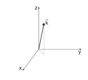
For a plane wave with vector wavenumber \(\vec{k}= \hat{\imath}+\hat{\jmath}+5\hat{k}\),
(a) Sketch a few of the planes of constant phase for this wave using 3-D Cartesian coordinates.
(b) Find the wavelength \(\lambda\) of this wave.
(c) Determine the minimum distance from the origin to the plane containing the point \((x=4, y=2, z=5)\) along the direction of \(\vec{k}\).
Begin by drawing 3-D Cartesian axes and the wavenumber vector \(\vec{k}= \hat{\imath}+\hat{\jmath}+5\hat{k}\), which should look something like this:
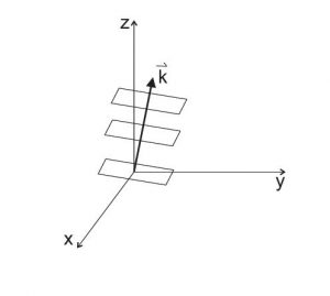
Remember that the planes of constant phase are perpendicular to the propagation vector \(\vec{k}\); here are some examples:
The relationship between the magnitude of the 3-D wavenumber \(|\vec{k}|\) and the wavelength \(\lambda\) is given by Eq. 3.45:
\begin{equation*}
|\vec{k}|=\sqrt{k_x^2+k_y^2+k_z^2}=\frac{2\pi}{\lambda}.
\end{equation*}
Solving Eq. 3.45 for \(\lambda\) gives
\begin{align*}
\lambda&=\frac{2\pi}{|\vec{k}|}=\frac{2\pi}{\sqrt{k_x^2+k_y^2+k_z^2}}\\
&=\frac{2\pi}{\sqrt{1^2+1^2+5^2}}=\frac{2\pi}{\sqrt{27}}=1.21 \textrm{ units}
\end{align*}
in which the units will be meters if the wavenumber components \(k_x\), \(k_y\), and \(k_z\) have units of radians per meter.
As explained in Section 3.4, for all points in a given plane of constant phase, the dot product between the vector \(\vec{k}\) and the position vector \(\vec{r}\) to any one of those points has a constant value. Here’s a sketch of the position vector \(\vec{r}\) to the point (4,2,5):
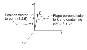
and although every point in the plane has a different position vector, the component of those position vectors in the direction of \(\vec{k}\) is the same. That component is \(|\vec{r}|\cos{\theta}\), in which \(\theta\) is the angle between \(\vec{k}\) and \(\vec{r}\).
Recall that the dot product \(\vec{k}\circ \vec{r}\) equals \(|\vec{k}||\vec{r}|\cos{\theta}\), so dividing that product by the magnitude of \(\vec{k}\) gives \(|\vec{r}|\cos{\theta}\), which is the distance from the origin to the plane containing the point with position vector \(\vec{r}\).
Note also that the components of the vector \(\vec{r}\) from point (\(x_1\), \(y_1\), \(z_1\)) to point (\(x_2\), \(y_2\), \(z_2\)) can be found using
\begin{equation*}
\vec{r}=(x_2-x_1)\hat{\imath}+(y_2-y_1)\hat{\jmath}+(z_2-z_1)\hat{k}
\end{equation*}
so the vector \(\vec{r}\) from the origin to point (4,2,5) is given by
\begin{equation*}
\vec{r}=(4-0)\hat{\imath}+(2-0)\hat{\jmath}+(5-0)\hat{k}=4\hat{\imath}+2\hat{\jmath}+5\hat{k}.
\end{equation*}
Plugging in the values for vectors \(\vec{r}\) and \(\vec{k}\) gives
\begin{align*}
\textrm{Distance to plane}&=\frac{\vec{k}\circ \vec{r}}{|\vec{k}|}\\
&=\frac{(\hat{\imath}+\hat{\jmath}+5\hat{k})\circ (4\hat{\imath}+2\hat{\jmath}+5\hat{k})}{\sqrt{1^2+1^2+5^2}}\\
&=\frac{4+2+25}{\sqrt{27}}=5.97 \textrm{ units}
\end{align*}
in which the units are the units of the position vector \(\vec{r}\).
Part (a):
Full Solution: Begin by drawing 3-D Cartesian axes and the wavenumber vector \(\vec{k}= \hat{\imath}+\hat{\jmath}+5\hat{k}\), which should look something like this:
Remember that the planes of constant phase are perpendicular to the propagation vector \(\vec{k}\); here are some examples:
Part (b):
The relationship between the magnitude of the 3-D wavenumber \(|\vec{k}|\) and the wavelength \(\lambda\) is given by Eq. 3.45:
\begin{equation*}
|\vec{k}|=\sqrt{k_x^2+k_y^2+k_z^2}=\frac{2\pi}{\lambda}.
\end{equation*}
Solving Eq. 3.45 for \(\lambda\) gives
\begin{align*}
\lambda&=\frac{2\pi}{|\vec{k}|}=\frac{2\pi}{\sqrt{k_x^2+k_y^2+k_z^2}}\\
&=\frac{2\pi}{\sqrt{1^2+1^2+5^2}}=\frac{2\pi}{\sqrt{27}}=1.21 \textrm{ units}
\end{align*}
in which the units will be meters if the wavenumber components \(k_x\), \(k_y\), and \(k_z\) have units of radians per meter.
Part (c):
As explained in Section 3.4, for all points in a given plane of constant phase, the dot product between the vector \(\vec{k}\) and the position vector \(\vec{r}\) to any one of those points has a constant value. Here’s a sketch of the position vector \(\vec{r}\) to the point (4,2,5):
and although every point in the plane has a different position vector, the component of those position vectors in the direction of \(\vec{k}\) is the same. That component is \(|\vec{r}|\cos{\theta}\), in which \(\theta\) is the angle between \(\vec{k}\) and \(\vec{r}\).
Recall that the dot product \(\vec{k}\circ \vec{r}\) equals \(|\vec{k}||\vec{r}|\cos{\theta}\), so dividing that product by the magnitude of \(\vec{k}\) gives \(|\vec{r}|\cos{\theta}\), which is the distance from the origin to the plane containing the point with position vector \(\vec{r}\).
Note also that the components of the vector \(\vec{r}\) from point \((x_1\), \(y_1\), \(z_1\)) to point \((x_2\), \(y_2\), \(z_2\)) can be found using
\begin{equation*}
\vec{r}=(x_2-x_1)\hat{\imath}+(y_2-y_1)\hat{\jmath}+(z_2-z_1)\hat{k}
\end{equation*}
so the vector \(\vec{r}\) from the origin to point (4,2,5) is given by
\begin{equation*}
\vec{r}=(4-0)\hat{\imath}+(2-0)\hat{\jmath}+(5-0)\hat{k}=4\hat{\imath}+2\hat{\jmath}+5\hat{k}.
\end{equation*}
Plugging in the values for vectors \(\vec{r}\) and \(\vec{k}\) gives
\begin{align*}
\textrm{Distance to plane}&=\frac{\vec{k}\circ \vec{r}}{|\vec{k}|}\\
&=\frac{(\hat{\imath}+\hat{\jmath}+5\hat{k})\circ (4\hat{\imath}+2\hat{\jmath}+5\hat{k})}{\sqrt{1^2+1^2+5^2}}\\
&=\frac{4+2+25}{\sqrt{27}}=5.97 \textrm{ units}
\end{align*}
in which the units are the units of the position vector \(\vec{r}\).
For the 2-D Gaussian wavefunction \(f(x,y)=Ae^{-\left[\frac{(x-x_0)^2}{2\sigma_x^2}+\frac{(y-y_0)^2}{2\sigma_y^2}\right]}\), show that
(a) The gradient \(\vec{\nabla}f\) is zero at the peak of the function \(x=x_0\), \(y=y_0\).
(b) The Laplacian \(\nabla^2f\) is negative at the location of the peak.
(c) The sharper the peak (smaller \(\sigma_x\) and \(\sigma_y\)), the larger the Laplacian.
The gradient in 3-D Cartesian coordinates is defined in Eq. 3.53 as
\begin{equation*}
\vec{\nabla}=\hat{\imath}\frac{\partial}{\partial x}+\hat{\jmath}\frac{\partial}{\partial y}+\hat{k}\frac{\partial}{\partial z},
\end{equation*}
and in 2-D Cartesian coordinates the gradient is the first two terms:
\begin{equation*}
\vec{\nabla}=\hat{\imath}\frac{\partial}{\partial x}+\hat{\jmath}\frac{\partial}{\partial y}.
\end{equation*}
Applying the 2-D Cartesian gradient from the previous hint to the 2-D Gaussian wavefunction \(f(x,y)\) gives
\begin{equation*}
\vec{\nabla}f(x,y)=\left(\hat{\imath}\frac{\partial}{\partial x}+\hat{\jmath}\frac{\partial}{\partial y}\right)Ae^{-\left[\frac{(x-x_0)^2}{2\sigma_x^2}+\frac{(y-y_0)^2}{2\sigma_y^2}\right]}.
\end{equation*}
The partial derivatives in the previous hint are
\begin{equation*}
\frac{\partial \left(Ae^{-\left[\frac{(x-x_0)^2}{2\sigma_x^2}+\frac{(y-y_0)^2}{2\sigma_y^2}\right]}\right)}{\partial x}=-\frac{2(x-x_0)}{2\sigma_x^2}Ae^{-\left[\frac{(x-x_0)^2}{2\sigma_x^2}+\frac{(y-y_0)^2}{2\sigma_y^2}\right]}
\end{equation*}
and
\begin{equation*}
\frac{\partial \left(Ae^{-\left[\frac{(x-x_0)^2}{2\sigma_x^2}+\frac{(y-y_0)^2}{2\sigma_y^2}\right]}\right)}{\partial y}=-\frac{2(y-y_0)}{2\sigma_y^2}Ae^{-\left[\frac{(x-x_0)^2}{2\sigma_x^2}+\frac{(y-y_0)^2}{2\sigma_y^2}\right]}.
\end{equation*}
And plugging in the values \(x=x_0\) and \(y=y_0\) yields the desired result.
The Laplacian \(\nabla^2f\) in 3-D Cartesian coordinates is defined in Eq. 3.49:
\begin{equation*}
\nabla^2=\frac{\partial^2 }{\partial x^2}+\frac{\partial^2}{\partial y^2}+\frac{\partial^2}{\partial z^2},
\end{equation*}
and in 2-D Cartesian coordinates, the Laplacian is the first two terms:
\begin{equation*}
\nabla^2=\frac{\partial^2 }{\partial x^2}+\frac{\partial^2}{\partial y^2}.
\end{equation*}
Applying the 2-D Cartesian Laplacian from the previous hint to the 2-D Gaussian wavefunction \(f(x,y)\) gives
\begin{equation*}
\nabla^2f(x,y)=\left(\frac{\partial^2 }{\partial x^2}+\frac{\partial^2}{\partial y^2}\right)Ae^{-\left[\frac{(x-x_0)^2}{2\sigma_x^2}+\frac{(y-y_0)^2}{2\sigma_y^2}\right]}.
\end{equation*}
The partial derivatives in the previous hint are
\begin{align*}
\frac{\partial^2 \left(Ae^{-\left[\frac{(x-x_0)^2}{2\sigma_x^2}+\frac{(y-y_0)^2}{2\sigma_y^2}\right]}\right)}{\partial x^2}&=\frac{\partial}{\partial x}\left[-\frac{2(x-x_0)}{2\sigma_x^2}Ae^{-\left[\frac{(x-x_0)^2}{2\sigma_x^2}+\frac{(y-y_0)^2}{2\sigma_y^2}\right]}\right]\\
&=\left[\frac{-1}{\sigma_x^2}+\frac{(x-x_0)^2}{\sigma_x^4}\right]Ae^{-\left[\frac{(x-x_0)^2}{2\sigma_x^2}+\frac{(y-y_0)^2}{2\sigma_y^2}\right]}
\end{align*}
and
\begin{align*}
\frac{\partial^2 \left(Ae^{-\left[\frac{(x-x_0)^2}{2\sigma_x^2}+\frac{(y-y_0)^2}{2\sigma_y^2}\right]}\right)}{\partial y^2}&=\frac{\partial}{\partial y}\left[-\frac{2(y-y_0)}{2\sigma_y^2}Ae^{-\left[\frac{(x-x_0)^2}{2\sigma_x^2}+\frac{(y-y_0)^2}{2\sigma_y^2}\right]}\right]\\
&=\left[\frac{-1}{\sigma_y^2}+\frac{(y-y_0)^2}{\sigma_y^4}\right]Ae^{-\left[\frac{(x-x_0)^2}{2\sigma_x^2}+\frac{(y-y_0)^2}{2\sigma_y^2}\right]}.
\end{align*}
Once again, plugging in the values \(x=x_0\) and \(y=y_0\) yields the desired result.
Consider the result of Part (b) at the peak \(x=x_0\) and \(y=y_0\):
\begin{equation*}
\nabla^2f(x,y)=A\left(\frac{-1}{\sigma_x^2}+\frac{-1}{\sigma_y^2}\right)
\end{equation*}
which determines the sign of the Laplacian \(\nabla^2f(x,y)\) at the peak as well as the dependence of the Laplacian on the width of the peak \(\sigma_x\) and \(\sigma_y\).
Part (a):
The gradient in 3-D Cartesian coordinates is defined in Eq. 3.53 as
\begin{equation*}
\vec{\nabla}=\hat{\imath}\frac{\partial}{\partial x}+\hat{\jmath}\frac{\partial}{\partial y}+\hat{k}\frac{\partial}{\partial z},
\end{equation*}
and in 2-D Cartesian coordinates the gradient is the first two terms:
\begin{equation*}
\vec{\nabla}=\hat{\imath}\frac{\partial}{\partial x}+\hat{\jmath}\frac{\partial}{\partial y}.
\end{equation*}
Applying the 2-D Cartesian gradient to the 2-D Gaussian wavefunction \(f(x,y)\) gives
\begin{equation*}
\vec{\nabla}f(x,y)=\left(\hat{\imath}\frac{\partial}{\partial x}+\hat{\jmath}\frac{\partial}{\partial y}\right)Ae^{-\left[\frac{(x-x_0)^2}{2\sigma_x^2}+\frac{(y-y_0)^2}{2\sigma_y^2}\right]},
\end{equation*}
and the partial derivatives in the previous hint are
\begin{equation*}
\frac{\partial \left(Ae^{-\left[\frac{(x-x_0)^2}{2\sigma_x^2}+\frac{(y-y_0)^2}{2\sigma_y^2}\right]}\right)}{\partial x}=-\frac{2(x-x_0)}{2\sigma_x^2}Ae^{-\left[\frac{(x-x_0)^2}{2\sigma_x^2}+\frac{(y-y_0)^2}{2\sigma_y^2}\right]}
\end{equation*}
and
\begin{equation*}
\frac{\partial \left(Ae^{-\left[\frac{(x-x_0)^2}{2\sigma_x^2}+\frac{(y-y_0)^2}{2\sigma_y^2}\right]}\right)}{\partial y}=-\frac{2(y-y_0)}{2\sigma_y^2}Ae^{-\left[\frac{(x-x_0)^2}{2\sigma_x^2}+\frac{(y-y_0)^2}{2\sigma_y^2}\right]}.
\end{equation*}
Plugging in the values \(x=x_0\) and \(y=y_0\) yields the result \(\vec{\nabla}f(x,y)=0\) at the peak of the Gaussian function.
Part (b):
The Laplacian \(\nabla^2f\) in 3-D Cartesian coordinates is defined in Eq. 3.49:
\begin{equation*}
\nabla^2=\frac{\partial^2 }{\partial x^2}+\frac{\partial^2}{\partial y^2}+\frac{\partial^2}{\partial z^2},
\end{equation*}
and in 2-D Cartesian coordinates, the Laplacian is the first two terms:
\begin{equation*}
\nabla^2=\frac{\partial^2 }{\partial x^2}+\frac{\partial^2}{\partial y^2}.
\end{equation*}
Applying the 2-D Cartesian Laplacian to the 2-D Gaussian wavefunction \(f(x,y)\) gives
\begin{equation*}
\nabla^2f(x,y)=\left(\frac{\partial^2 }{\partial x^2}+\frac{\partial^2}{\partial y^2}\right)Ae^{-\left[\frac{(x-x_0)^2}{2\sigma_x^2}+\frac{(y-y_0)^2}{2\sigma_y^2}\right]}.
\end{equation*}
These partial derivatives are
\begin{align*}
\frac{\partial^2 \left(Ae^{-\left[\frac{(x-x_0)^2}{2\sigma_x^2}+\frac{(y-y_0)^2}{2\sigma_y^2}\right]}\right)}{\partial x^2}&=\frac{\partial}{\partial x}\left[-\frac{2(x-x_0)}{2\sigma_x^2}Ae^{-\left[\frac{(x-x_0)^2}{2\sigma_x^2}+\frac{(y-y_0)^2}{2\sigma_y^2}\right]}\right]\\
&=\left[\frac{-1}{\sigma_x^2}+\frac{(x-x_0)^2}{\sigma_x^4}\right]Ae^{-\left[\frac{(x-x_0)^2}{2\sigma_x^2}+\frac{(y-y_0)^2}{2\sigma_y^2}\right]}
\end{align*}
and
\begin{align*}
\frac{\partial^2 \left(Ae^{-\left[\frac{(x-x_0)^2}{2\sigma_x^2}+\frac{(y-y_0)^2}{2\sigma_y^2}\right]}\right)}{\partial y^2}&=\frac{\partial}{\partial y}\left[-\frac{2(y-y_0)}{2\sigma_y^2}Ae^{-\left[\frac{(x-x_0)^2}{2\sigma_x^2}+\frac{(y-y_0)^2}{2\sigma_y^2}\right]}\right]\\
&=\left[\frac{-1}{\sigma_y^2}+\frac{(y-y_0)^2}{\sigma_y^4}\right]Ae^{-\left[\frac{(x-x_0)^2}{2\sigma_x^2}+\frac{(y-y_0)^2}{2\sigma_y^2}\right]}.
\end{align*}
Once again, plugging in the values \(x=x_0\) and \(y=y_0\) yields the desired result, since this expression must be negative.
Part (c):
Consider the result of Part (b) at the peak \(x=x_0\) and \(y=y_0\):
\begin{equation*}
\nabla^2f(x,y)=A\left(\frac{-1}{\sigma_x^2}+\frac{-1}{\sigma_y^2}\right)
\end{equation*}
which shows that the sign of the Laplacian \(\nabla^2f(x,y)\) at the peak is negative, and that a sharper peak (smaller values of \(\sigma_x\) and \(\sigma_y\)) has a larger value of the Laplacian.
Show that in a region of constant potential \(V\)
\begin{equation*}
\Psi_n(x,y,z,t)=\sqrt{\frac{8}{a_x a_y a_z}}\sin{\left(k_{n,x}x\right)}\sin{\left(k_{n,y}y\right)}\sin{\left(k_{n,z}z\right)}e^{-iE_n t/\hbar}
\end{equation*}
is a solution to the Schrödinger equation in 3-D Cartesian coordinates if \(E_n=\frac{k_n^2 \hbar^2}{2m}\), with
\begin{equation*}
k_n^2=(k_{n,x})^2+(k_{n,y})^2+(k_{n,z})^2
\end{equation*}
and
\begin{equation*}
k_{n,x}=\frac{n_x\pi}{a_x}\hspace{0.5cm}k_{n,y}=\frac{n_y\pi}{a_y}\hspace{0.5cm}k_{n,z}=\frac{n_z\pi}{a_z}.
\end{equation*}
To show that the function \(\Psi_n(x,y,z,t)\) is a solution to the 3-D time-dependent Schrödinger equation, plug the function into the Cartesian version of Eq. 3.50:
\begin{equation*}
i\hbar\frac{\partial \Psi(x,y,z,t)}{\partial t}=-\frac{\hbar^2}{2m}\nabla^2\Psi(x,y,z,t)
\end{equation*}
in which the constant value of potential \(V\) has been set to zero by choosing the appropriate reference level.
Taking the time derivative of \(\Psi_n(x,y,z,t)\) gives
\begin{align*}
\frac{\partial \Psi}{\partial t}&=\frac{\partial}{\partial t}\left[\sqrt{\frac{8}{a_x a_y a_z}}\sin{\left(k_{n,x}x\right)}\sin{\left(k_{n,y}y\right)}\sin{\left(k_{n,z}z\right)}e^{-iE_n t/\hbar}\right]\\
&=\frac{-iE_n}{\hbar}\left[\sqrt{\frac{8}{a_x a_y a_z}}\sin{\left(k_{n,x}x\right)}\sin{\left(k_{n,y}y\right)}\sin{\left(k_{n,z}z\right)}e^{-iE_n t/\hbar}\right]\\
&=\frac{-iE_n}{\hbar}\Psi.
\end{align*}
Taking the first x-spatial derivatives of \(\Psi_n(x,y,z,t)\) gives
\begin{align*}
\frac{\partial \Psi}{\partial x}&=\frac{\partial}{\partial x}\left[\sqrt{\frac{8}{a_x a_y a_z}}\sin{\left(k_{n,x}x\right)}\sin{\left(k_{n,y}y\right)}\sin{\left(k_{n,z}z\right)}e^{-iE_n t/\hbar}\right]\\
&=k_{n,x}\left[\sqrt{\frac{8}{a_x a_y a_z}}\cos{\left(k_{n,x}x\right)}\sin{\left(k_{n,y}y\right)}\sin{\left(k_{n,z}z\right)}e^{-iE_n t/\hbar}\right]
\end{align*}
and the second x-spatial derivative gives
\begin{align*}
\frac{\partial^2 \Psi}{\partial x^2}&=\frac{\partial}{\partial x}\left[k_{n,x}\sqrt{\frac{8}{a_x a_y a_z}}\cos{\left(k_{n,x}x\right)}\sin{\left(k_{n,y}y\right)}\sin{\left(k_{n,z}z\right)}e^{-iE_n t/\hbar}\right]\\
&=-(k_{n,x})^2\left[\sqrt{\frac{8}{a_x a_y a_z}}\sin{\left(k_{n,x}x\right)}\sin{\left(k_{n,y}y\right)}\sin{\left(k_{n,z}z\right)}e^{-iE_n t/\hbar}\right]\\
&=-(k_{n,x})^2\Psi.
\end{align*}
Taking the second y- and z-spatial derivatives gives
\begin{align*}
\frac{\partial^2 \Psi}{\partial y^2}&=-(k_{n,y})^2\left[\sqrt{\frac{8}{a_x a_y a_z}}\sin{\left(k_{n,x}x\right)}\sin{\left(k_{n,y}y\right)}\sin{\left(k_{n,z}z\right)}e^{-iE_n t/\hbar}\right]\\
&=-(k_{n,y})^2\Psi
\end{align*}
and
\begin{align*}
\frac{\partial^2 \Psi}{\partial z^2}&=-(k_{n,z})^2\left[\sqrt{\frac{8}{a_x a_y a_z}}\sin{\left(k_{n,x}x\right)}\sin{\left(k_{n,y}y\right)}\sin{\left(k_{n,z}z\right)}e^{-iE_n t/\hbar}\right]\\
&=-(k_{n,z})^2\Psi.
\end{align*}
Plugging the results of the time and spatial derivatives into the Schrödinger equation gives
\begin{equation*}
i\hbar\frac{-iE_n}{\hbar}\Psi=-\frac{\hbar^2}{2m}\left[-(k_{n,x})^2-(k_{n,y})^2-(k_{n,z})^2\right]\Psi
\end{equation*}
or, if \(k_n^2=(k_{n,x})^2+(k_{n,y})^2+(k_{n,z})^2\)
\begin{equation*}
E_n\Psi=\frac{\hbar^2}{2m}\left[(k_n)^2\right]\Psi
\end{equation*}
which is satisfied if \(E_n=\frac{k_n^2 \hbar^2}{2m}\).
To show that the function \(\Psi_n(x,y,z,t)\) is a solution to the 3-D time-dependent Schrödinger equation, plug the function into the Cartesian version of Eq. 3.50:
\begin{equation*}
i\hbar\frac{\partial \Psi(x,y,z,t)}{\partial t}=-\frac{\hbar^2}{2m}\nabla^2\Psi(x,y,z,t).
\end{equation*}
in which the constant value of potential \(V\) has been set to zero by choosing the appropriate reference level.
Taking the time derivative of \(\Psi_n(x,y,z,t)\) gives
\begin{align*}
\frac{\partial \Psi}{\partial t}&=\frac{\partial}{\partial t}\left[\sqrt{\frac{8}{a_x a_y a_z}}\sin{\left(k_{n,x}x\right)}\sin{\left(k_{n,y}y\right)}\sin{\left(k_{n,z}z\right)}e^{-iE_n t/\hbar}\right]\\
&=\frac{-iE_n}{\hbar}\left[\sqrt{\frac{8}{a_x a_y a_z}}\sin{\left(k_{n,x}x\right)}\sin{\left(k_{n,y}y\right)}\sin{\left(k_{n,z}z\right)}e^{-iE_n t/\hbar}\right]\\
&=\frac{-iE_n}{\hbar}\Psi,
\end{align*}
and taking the first x-spatial derivatives of \(\Psi_n(x,y,z,t)\) gives
\begin{align*}
\frac{\partial \Psi}{\partial x}&=\frac{\partial}{\partial x}\left[\sqrt{\frac{8}{a_x a_y a_z}}\sin{\left(k_{n,x}x\right)}\sin{\left(k_{n,y}y\right)}\sin{\left(k_{n,z}z\right)}e^{-iE_n t/\hbar}\right]\\
&=k_{n,x}\left[\sqrt{\frac{8}{a_x a_y a_z}}\cos{\left(k_{n,x}x\right)}\sin{\left(k_{n,y}y\right)}\sin{\left(k_{n,z}z\right)}e^{-iE_n t/\hbar}\right].
\end{align*}
The second x-spatial derivative gives
\begin{align*}
\frac{\partial^2 \Psi}{\partial x^2}&=\frac{\partial}{\partial x}\left[k_{n,x}\sqrt{\frac{8}{a_x a_y a_z}}\cos{\left(k_{n,x}x\right)}\sin{\left(k_{n,y}y\right)}\sin{\left(k_{n,z}z\right)}e^{-iE_n t/\hbar}\right]\\
&=-(k_{n,x})^2\left[\sqrt{\frac{8}{a_x a_y a_z}}\sin{\left(k_{n,x}x\right)}\sin{\left(k_{n,y}y\right)}\sin{\left(k_{n,z}z\right)}e^{-iE_n t/\hbar}\right]\\
&=-(k_{n,x})^2\Psi,
\end{align*}
and taking the second y- and z-spatial derivatives gives
\begin{align*}
\frac{\partial^2 \Psi}{\partial y^2}&=-(k_{n,y})^2\left[\sqrt{\frac{8}{a_x a_y a_z}}\sin{\left(k_{n,x}x\right)}\sin{\left(k_{n,y}y\right)}\sin{\left(k_{n,z}z\right)}e^{-iE_n t/\hbar}\right]\\
&=-(k_{n,y})^2\Psi
\end{align*}
and
\begin{align*}
\frac{\partial^2 \Psi}{\partial z^2}&=-(k_{n,z})^2\left[\sqrt{\frac{8}{a_x a_y a_z}}\sin{\left(k_{n,x}x\right)}\sin{\left(k_{n,y}y\right)}\sin{\left(k_{n,z}z\right)}e^{-iE_n t/\hbar}\right]\\
&=-(k_{n,z})^2\Psi.
\end{align*}
Plugging the results of the time and spatial derivatives into the Schrödinger equation gives
\begin{equation*}
i\hbar\frac{-iE_n}{\hbar}\Psi=-\frac{\hbar^2}{2m}\left[-(k_{n,x})^2-(k_{n,y})^2-(k_{n,z})^2\right]\Psi
\end{equation*}
or, if \(k_n^2=(k_{n,x})^2+(k_{n,y})^2+(k_{n,z})^2\)
\begin{equation*}
E_n\Psi=\frac{\hbar^2}{2m}\left[(k_n)^2\right]\Psi
\end{equation*}
which is satisfied if \(E_n=\frac{k_n^2 \hbar^2}{2m}\).
Use separation of variables to write the 3-D Schrödinger equation in spherical coordinates as two separate equations, one depending only on the radial coordinate \(r\) and the other depending only on the angular coordinates \(\theta\) and \(\phi\), with the potential energy depending only on the radial coordinate (so \(V=V(r)\))
The 3-D time-independent Schrödinger equation is given by Eq. 3.57 as
\begin{equation*}
-\frac{\hbar^2}{2m}\nabla^2 [\psi(\vec{r})]+V[\psi(\vec{r})]=E[\psi(\vec{r})]
\end{equation*}
and the Laplacian in spherical coordinates is given by Eq. 3.59 as
\begin{equation*}
\nabla^2=\frac{1}{r^2}\frac{\partial}{\partial r}\left(r^2\frac{\partial}{\partial r}\right)+\frac{1}{r^2\sin{\theta}}\frac{\partial}{\partial \theta}\left(\sin{\theta}\frac{\partial}{\partial \theta}\right)+\frac{1}{r^2\sin^2{\theta}}\frac{\partial^2}{\partial \phi^2}.
\end{equation*}
Write the spatial wavefunction \(\psi(\vec{r})\) as the product of two functions, one depending only on radial distance \(r\) (call it \(R(r)\)), and the other depending only on the angles \(\theta\) and \(\phi\) (call it \(Y(\theta, \phi))\):
\begin{equation*}
\psi(r,\theta,\phi)=R(r)Y(\theta,\phi)
\end{equation*}
and plug this into the spherical Schrödinger equation (start by operating on \(\psi(r, \theta, \phi)\) with the spherical Laplacian).
The spherical Laplacian operating on \(\psi(r, \theta, \phi)=R(r)Y(\theta, \phi)\) looks like this:
\begin{align*}
\nabla^2\psi(r,\theta,\phi)&=\nabla^2[R(r)Y(\theta,\phi)]\\
&=\frac{1}{r^2}\frac{\partial}{\partial r}\left(r^2\frac{\partial (RY)}{\partial r}\right)\\
&\hspace{0.25cm}+\frac{1}{r^2\sin{\theta}}\frac{\partial}{\partial \theta}\left(\sin{\theta}\frac{\partial (RY)}{\partial \theta}\right)+\frac{1}{r^2\sin^2{\theta}}\frac{\partial^2 (RY)}{\partial \phi^2}
\end{align*}
or
\begin{align*}
\nabla^2[R(r)Y(\theta,\phi)]&=\frac{Y}{r^2}\frac{d}{dr}\left(r^2\frac{dR}{dr}\right)\\
&\hspace{0.25cm}+\frac{R}{r^2\sin{\theta}}\frac{\partial}{\partial \theta}\left(\sin{\theta}\frac{\partial Y}{\partial \theta}\right)+\frac{R}{r^2\sin^2{\theta}}\frac{\partial^2 Y}{\partial \phi^2}.
\end{align*}
Note that the function \(Y(\theta,\phi)\) comes right out of the \(r\)-derivatives and that the function \(R(r)\) comes out of the \(\theta-\) and \(\phi-\)derivatives. Note also that the partial derivaties with respect to \(r\) become full derivatives when operating on the function \(R(r)\), since that function depends on only one variable \(r\).
Plugging the result from the previous hint into the spherical Schrödinger equation gives
\begin{align*}
&-\frac{\hbar^2}{2m}\left[\frac{Y}{r^2}\frac{d}{dr}\left(r^2\frac{dR}{dr}\right)+\frac{R}{r^2\sin{\theta}}\frac{\partial}{\partial \theta}\left(\sin{\theta}\frac{\partial Y}{\partial \theta}\right)+\frac{R}{r^2\sin^2{\theta}}\frac{\partial^2 Y}{\partial \phi^2} \right]\\
&\hspace{8cm}+V(RY)=E(RY)
\end{align*}
Now divide by \(RY\) and multiply by \(r^2\):
\begin{align*}
&-\frac{\hbar^2}{2m}\left[\frac{1}{R}\frac{d}{dr}\left(r^2\frac{dR}{dr}\right)+\frac{1}{Y\sin{\theta}}\frac{\partial}{\partial \theta}\left(\sin{\theta}\frac{\partial Y}{\partial \theta}\right)+\frac{1}{Y\sin^2{\theta}}\frac{\partial^2 Y}{\partial \phi^2} \right]\\
&\hspace{8cm}+(V-E)r^2=0
\end{align*}
and gather the terms that depend on \(r\) on one side of the equation and those that depend on \(\theta\) and \(\phi\) on the other side:
\begin{align*}
&\frac{\hbar^2}{2m}\frac{1}{R}\frac{d}{dr}\left(r^2\frac{dR}{dr}\right)-(V-E)r^2=\\
&\frac{1}{Y\sin{\theta}}\frac{\partial}{\partial \theta}\left(\sin{\theta}\frac{\partial Y}{\partial \theta}\right)+\frac{1}{Y\sin^2{\theta}}\frac{\partial^2 Y}{\partial \phi^2}
\end{align*}
Note that the left side of this equation depends only on \(r\), since the problem statement says that the potential \(V\) is a function only of distance, not angle. Note also that the right side depends only on the angles \(\theta\) and \(\phi\), not on \(r\). Hence this equation can be true only if both sides are constant, by the same logic used in the text for separating the time and spatial portions of the wavefunction.
The separated equations are
\begin{equation*}
\frac{\hbar^2}{2m}\frac{1}{R}\frac{d}{dr}\left(r^2\frac{dR}{dr}\right)-(V-E)r^2=\textrm{ constant}
\end{equation*}
and
\begin{equation*}
\frac{1}{Y\sin{\theta}}\frac{\partial}{\partial \theta}\left(\sin{\theta}\frac{\partial Y}{\partial \theta}\right)+\frac{1}{Y\sin^2{\theta}}\frac{\partial^2 Y}{\partial \phi^2}=\textrm{ constant}.
\end{equation*}
The 3-D time-independent Schrödinger equation is given by Eq. 3.57 as
\begin{equation*}
-\frac{\hbar^2}{2m}\nabla^2 [\psi(\vec{r})]+V[\psi(\vec{r})]=E[\psi(\vec{r})]
\end{equation*}
and the Laplacian in spherical coordinates is given by Eq. 3.59 as
\begin{equation*}
\nabla^2=\frac{1}{r^2}\frac{\partial}{\partial r}\left(r^2\frac{\partial}{\partial r}\right)+\frac{1}{r^2\sin{\theta}}\frac{\partial}{\partial \theta}\left(\sin{\theta}\frac{\partial}{\partial \theta}\right)+\frac{1}{r^2\sin^2{\theta}}\frac{\partial^2}{\partial \phi^2}.
\end{equation*}
Write the spatial wavefunction \(\psi(\vec{r})\) as the product of two functions, one depending only on radial distance \(r\) (call it \(R(r)\)), and the other depending only on the angles \(\theta\) and \(\phi\) (call it \(Y(\theta,\phi))\):
\begin{equation*}
\psi(r,\theta,\phi)=R(r)Y(\theta,\phi)
\end{equation*}
and plug this into the spherical Schrödinger equation (start by operating on \(\psi(r,\theta,\phi)\) with the spherical Laplacian). The spherical Laplacian operating on \(\psi(r,\theta,\phi)=R(r)Y(\theta,\phi)\) looks like this:
\begin{align*}
\nabla^2\psi(r,\theta,\phi)&=\nabla^2[R(r)Y(\theta,\phi)]\\
&=\frac{1}{r^2}\frac{\partial}{\partial r}\left(r^2\frac{\partial (RY)}{\partial r}\right)\\
&\hspace{0.25cm}+\frac{1}{r^2\sin{\theta}}\frac{\partial}{\partial \theta}\left(\sin{\theta}\frac{\partial (RY)}{\partial \theta}\right)+\frac{1}{r^2\sin^2{\theta}}\frac{\partial^2 (RY)}{\partial \phi^2}
\end{align*}
or
\begin{align*}
\nabla^2[R(r)Y(\theta,\phi)]&=\frac{Y}{r^2}\frac{d}{dr}\left(r^2\frac{dR}{dr}\right)\\
&\hspace{0.25cm}+\frac{R}{r^2\sin{\theta}}\frac{\partial}{\partial \theta}\left(\sin{\theta}\frac{\partial Y}{\partial \theta}\right)+\frac{R}{r^2\sin^2{\theta}}\frac{\partial^2 Y}{\partial \phi^2}.
\end{align*}
Note that the function \(Y(\theta,\phi)\) comes right out of the \(r\)-derivatives and that the function \(R(r)\) comes out of the \(\theta-\) and \(\phi-\)derivatives. Note also that the partial derivaties with respect to \(r\) become full derivatives when operating on the function \(R(r)\), since that function depends on only one variable \(r\).
Plugging this result into the spherical Schrödinger equation gives
\begin{align*}
&-\frac{\hbar^2}{2m}\left[\frac{Y}{r^2}\frac{d}{dr}\left(r^2\frac{dR}{dr}\right)+\frac{R}{r^2\sin{\theta}}\frac{\partial}{\partial \theta}\left(\sin{\theta}\frac{\partial Y}{\partial \theta}\right)+\frac{R}{r^2\sin^2{\theta}}\frac{\partial^2 Y}{\partial \phi^2} \right]\\
&\hspace{8cm}+V(RY)=E(RY)
\end{align*}
Now divide by \(RY\) and multiply by \(r^2\):
\begin{align*}
&-\frac{\hbar^2}{2m}\left[\frac{1}{R}\frac{d}{dr}\left(r^2\frac{dR}{dr}\right)+\frac{1}{Y\sin{\theta}}\frac{\partial}{\partial \theta}\left(\sin{\theta}\frac{\partial Y}{\partial \theta}\right)+\frac{1}{Y\sin^2{\theta}}\frac{\partial^2 Y}{\partial \phi^2} \right]\\
&\hspace{8cm}+(V-E)r^2=0
\end{align*}
and gather the terms that depend on \(r\) on one side of the equation and those that depend on \(\theta\) and \(\phi\) on the other side:
\begin{align*}
&\frac{\hbar^2}{2m}\frac{1}{R}\frac{d}{dr}\left(r^2\frac{dR}{dr}\right)-(V-E)r^2=\\
&\frac{1}{Y\sin{\theta}}\frac{\partial}{\partial \theta}\left(\sin{\theta}\frac{\partial Y}{\partial \theta}\right)+\frac{1}{Y\sin^2{\theta}}\frac{\partial^2 Y}{\partial \phi^2}
\end{align*}
Note that the left side of this equation depends only on \(r\), since the problem statement says that the potential \(V\) is a function only of distance, not angle. Note also that the right side depends only on the angles \(\theta\) and \(\phi\), not on \(r\). Hence this equation can be true only if both sides are constant, by the same logic used in the text for separating the time and spatial portions of the wavefunction.
Thus the separated equations are
\begin{equation*}
\frac{\hbar^2}{2m}\frac{1}{R}\frac{d}{dr}\left(r^2\frac{dR}{dr}\right)-(V-E)r^2=\textrm{ constant}
\end{equation*}
and
\begin{equation*}
\frac{1}{Y\sin{\theta}}\frac{\partial}{\partial \theta}\left(\sin{\theta}\frac{\partial Y}{\partial \theta}\right)+\frac{1}{Y\sin^2{\theta}}\frac{\partial^2 Y}{\partial \phi^2}=\textrm{ constant}.
\end{equation*}
Show that the function \(R(r)=\frac{1}{r\sqrt{2\pi a}}\sin\left(\frac{n\pi r}{a}\right)\) is a solution to the radial portion of the 3-D Schrödinger equation in spherical coordinates for \(V=0\) and with separation constant \(E_n=\frac{n^2 \pi^2 \hbar^2}{2ma^2}\).
The radial portion of the 3-D Schrödinger equation in spherical coordinates is given in Problem 9 as
\begin{equation*}
\frac{\hbar^2}{2m}\frac{1}{R}\frac{d}{dr}\left(r^2\frac{dR}{dr}\right)+E_nr^2=\textrm{ constant}
\end{equation*}
for a region in which \(V=0\).
To prove that the function \(R(r)=\frac{1}{r\sqrt{2\pi a}}\sin\left(\frac{n\pi r}{a}\right)\) is a solution to the radial equation, plug \(R(r)\) into the equation and verify that the terms on the left side produce a constant.
Taking the derivative of \(R(r)\) with respect to \(r\) gives
\begin{align*}
\frac{dR(r)}{dr}&=\frac{d\left[\frac{1}{r\sqrt{2\pi a}}\sin\left(\frac{n\pi r}{a}\right)\right]}{dr}\\
&=\frac{1}{\sqrt{2\pi a}}\left[-\frac{1}{r^2}\sin\left(\frac{n\pi r}{a}\right)+\frac{1}{r}\left(\frac{n\pi}{a}\right)\cos{\left(\frac{n\pi r}{a}\right)}\right]
\end{align*}
Multiplying \(\frac{\partial R(r)}{\partial r}\) by \(r^2\) gives
\begin{equation*}
r^2\frac{dR(r)}{dr}=-\frac{1}{\sqrt{2\pi a}}\left[\sin\left(\frac{n\pi r}{a}\right)-r\left(\frac{n\pi}{a}\right)\cos{\left(\frac{n\pi r}{a}\right)}\right]
\end{equation*}
and taking the derivative of this expression with respect to \(r\) gives
\begin{align*}
\frac{d}{dr}\left[r^2\frac{dR(r)}{dr}\right]&=-\frac{1}{\sqrt{2\pi a}}\left[\left(\frac{n\pi}{a}\right)\cos{\left(\frac{n\pi r}{a}\right)}\right.\\
&\hspace{0.25cm}\left.-\left(\frac{n\pi}{a}\right)\cos{\left(\frac{n\pi r}{a}\right)}+r\left(\frac{n\pi}{a}\right)^2\sin{\left(\frac{n\pi r}{a}\right)}\right]\\
&=-\frac{r}{\sqrt{2\pi a}}\left(\frac{n\pi}{a}\right)^2\sin{\left(\frac{n\pi r}{a}\right)}.
\end{align*}
Multiplying by \(\frac{1}{R}\) makes this
\begin{align*}
\frac{1}{R}\frac{d}{dr}\left[r^2\frac{dR(r)}{dr}\right]&=\frac{-\frac{r}{\sqrt{2\pi a}}\left(\frac{n\pi}{a}\right)^2\sin{\left(\frac{n\pi r}{a}\right)}}{\frac{1}{r\sqrt{2\pi a}}\sin\left(\frac{n\pi r}{a}\right)}\\
&=-r^2\left(\frac{n\pi}{a}\right)^2.
\end{align*}
and multiplying by \(\frac{\hbar^2}{2m}\) gives the first term in the radial equation:
\begin{equation*}
\frac{\hbar^2}{2m}\frac{1}{R}\frac{d}{dr}\left[r^2\frac{dR(r)}{dr}\right]=-\frac{\hbar^2}{2m}\left(\frac{n\pi r}{a}\right)^2.
\end{equation*}
Inserting this expression into the radial equation gives
\begin{equation*}
-\frac{\hbar^2}{2m}\left(\frac{n\pi r}{a}\right)^2+E_nr^2=\textrm{ constant}
\end{equation*}
and inserting the expression for \(E_n\) given in the problem statement makes this
\begin{equation*}
-\frac{\hbar^2}{2m}\left(\frac{n\pi r}{a}\right)^2+\frac{n^2 \pi^2 \hbar^2}{2ma^2}r^2=\textrm{ constant}
\end{equation*}
which is true.
The radial portion of the 3-D Schrödinger equation in spherical coordinates is given in Problem 9 as
\begin{equation*}
\frac{\hbar^2}{2m}\frac{1}{R}\frac{d}{dr}\left(r^2\frac{dR}{dr}\right)+E_nr^2=\textrm{ constant}
\end{equation*}
for a region in which \(V=0\). To prove that the function \(R(r)=\frac{1}{r\sqrt{2\pi a}}\sin\left(\frac{n\pi r}{a}\right)\) is a solution to the radial equation, plug \(R(r)\) into the equation and verify that the terms on the left side produce a constant.
Taking the derivative of \(R(r)\) with respect to \(r\) gives
\begin{align*}
\frac{dR(r)}{dr}&=\frac{d\left[\frac{1}{r\sqrt{2\pi a}}\sin\left(\frac{n\pi r}{a}\right)\right]}{dr}\\
&=\frac{1}{\sqrt{2\pi a}}\left[-\frac{1}{r^2}\sin\left(\frac{n\pi r}{a}\right)+\frac{1}{r}\left(\frac{n\pi}{a}\right)\cos{\left(\frac{n\pi r}{a}\right)}\right]
\end{align*}
Multiplying \(\frac{\partial R(r)}{\partial r}\) by\(r^2\) gives
\begin{equation*}
r^2\frac{dR(r)}{dr}=-\frac{1}{\sqrt{2\pi a}}\left[\sin\left(\frac{n\pi r}{a}\right)-r\left(\frac{n\pi}{a}\right)\cos{\left(\frac{n\pi r}{a}\right)}\right]
\end{equation*}
and taking the derivative of this expression with respect to \(r\) gives
\begin{align*}
\frac{d}{dr}\left[r^2\frac{dR(r)}{dr}\right]&=-\frac{1}{\sqrt{2\pi a}}\left[\left(\frac{n\pi}{a}\right)\cos{\left(\frac{n\pi r}{a}\right)}\right.\\
&\hspace{0.25cm}\left.-\left(\frac{n\pi}{a}\right)\cos{\left(\frac{n\pi r}{a}\right)}+r\left(\frac{n\pi}{a}\right)^2\sin{\left(\frac{n\pi r}{a}\right)}\right]\\
&=-\frac{r}{\sqrt{2\pi a}}\left(\frac{n\pi}{a}\right)^2\sin{\left(\frac{n\pi r}{a}\right)}.
\end{align*}
Multiplying by \(\frac{1}{R}\) makes this
\begin{align*}
\frac{1}{R}\frac{d}{dr}\left[r^2\frac{dR(r)}{dr}\right]&=\frac{-\frac{r}{\sqrt{2\pi a}}\left(\frac{n\pi}{a}\right)^2\sin{\left(\frac{n\pi r}{a}\right)}}{\frac{1}{r\sqrt{2\pi a}}\sin\left(\frac{n\pi r}{a}\right)}\\
&=-r^2\left(\frac{n\pi}{a}\right)^2.
\end{align*}
and multiplying by \(\frac{\hbar^2}{2m}\) gives the first term in the radial equation:
\begin{equation*}
\frac{\hbar^2}{2m}\frac{1}{R}\frac{d}{dr}\left[r^2\frac{dR(r)}{dr}\right]=-\frac{\hbar^2}{2m}\left(\frac{n\pi r}{a}\right)^2.
\end{equation*}
Inserting this expression into the radial equation gives
\begin{equation*}
-\frac{\hbar^2}{2m}\left(\frac{n\pi r}{a}\right)^2+E_nr^2=\textrm{ constant}
\end{equation*}
and inserting the expression for \(E_n\) given in the problem statement makes this
\begin{equation*}
-\frac{\hbar^2}{2m}\left(\frac{n\pi r}{a}\right)^2+\frac{n^2 \pi^2 \hbar^2}{2ma^2}r^2=\textrm{ constant}
\end{equation*}
which is true.
After working through this chapter, readers will be able to use conservation of energy to justify the Schrödinger Equation, explain the physical meaning of each term of the Schrödinger Equation, use separation of variables to find the time-independent version of the Schrödinger Equation, and extend the one-dimensional Schrödinger Equation to three-dimensional situations.
Relate energy to frequency using the Planck-Einstein relation
Relate momentum to wavenumber using de Broglie’s relation
Use plane-wave function to relate frequency and wavenumber to time and space derivatives
Synthesize complex wavefunctions by weighted linear combination of plane waves
Explain the meaning of each term in the Schrödinger Equation
Explain why the Schrödinger Equation is a parabolic, second-order partial differential equation
Relate the curvature of a wavefunction to its variation over time
Use separation of variables to find the time-independent version of the Schrödinger Equation
Express the Schrödinger Equation as an eigenvalue equation using the Hamiltonian operator
Extend the one-dimensional Schrödinger Equation to three dimensions using the Laplacian operator
